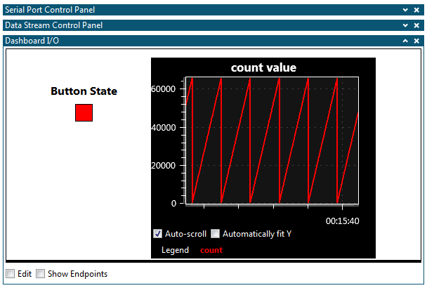
The purpose of this example is to show how to set up the configuration files required to automatically configure a dashboard with a signal showing the state of a pushbutton on the target hardware and a graph showing the value of a counter in the target application. The screenshot below shows the final dashboard.
The target code used in this example can be found in Auto-Configuration Example Code.
Three files are required by the Data Visualizer to enable Auto-Configuration, a .ds file describing the data stream content, a .db file describing the dashboard and a .sc file describing the connections between the data stream content and the dashboard elements. All files should be named "C0FFEEC0FFEEC0FFEEC0FFEE" before the extension to match the Auto Configuration ID sent by the application code.
The example application generates a data stream with two stream components, an unsigned 16-bit value and an unsigned 8-bit value.
- Create a file called
"C0FFEEC0FFEEC0FFEEC0FFEE.ds" and add the content
below
D,1,1,count
B,2,1,button
The .ds file will create a table with two sources from the data stream. Column 1 row 1 will contain a source with unsigned 16-bit values named "count" and column 2, row 1 will contain a source with unsigned 8-bit values named "button". For more information on the .ds file format see Configuration Format.
The easiest way to set up a dashboard for the Auto-Configuration is to draw it in the Data Visualizer GUI and save the configuration to file.
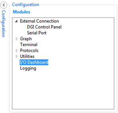
- Open the configuration panel
- Add a new I/O Dashboard component by double-clicking the I/O Dashboard module
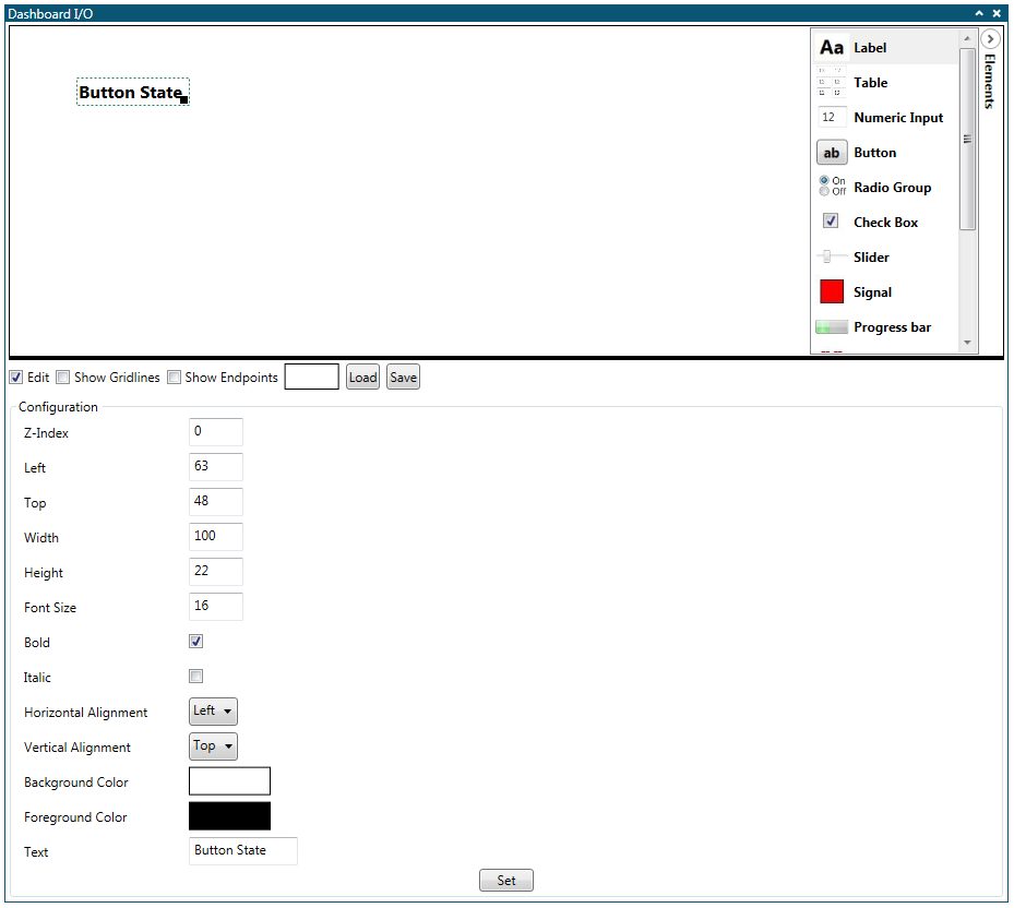
- Enable editing the dashboard by clicking the Edit option in the lower left corner of the Dashboard I/O module
- Open the Elements panel in the upper right corner of the dashboard and drag elements onto the dashboard.
- Drag a Label element to the dashboard
- Select the Label element and set Font Size to 16, Tick the Bold option, set Text field to “Button State” and set Width to 100.
- Push Set
- Drag a Signal element to the Dashboard and put it below the Button State label
- Drag a Graph element to the Dashboard and put it to the right of the Button State label and signal
- Select the Graph element and set Title to “count value”, X Maximum to 5, Y Maximum to 66000
- Click Set
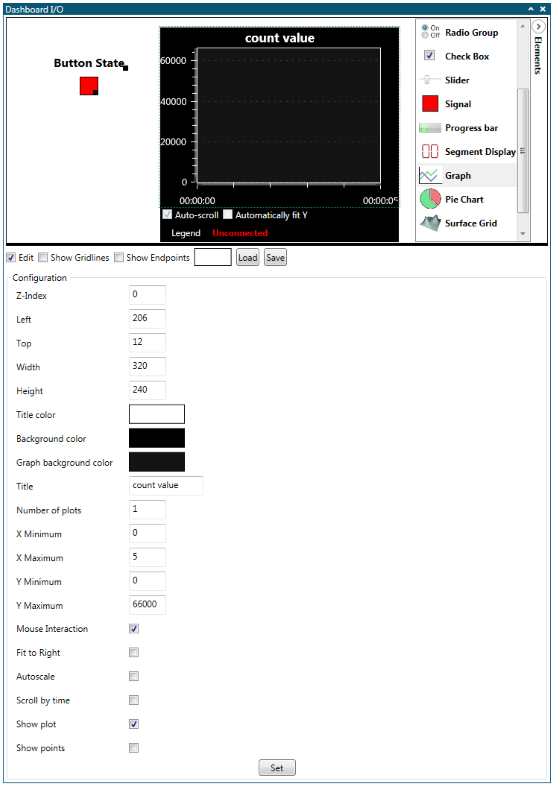
- Click Save
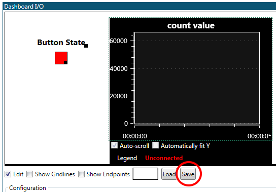
- Save the Dashboard configuration as “C0FFEEC0FFEEC0FFEEC0FFEE.db” in the same folder as the .ds file
The .db file content should have content similar to:
{
0,
'\0',
0, 255, 255, 255,
44, 1,
};

{
0, // Dashboard ID
0, // Element ID
DB_TYPE_LABEL, // Element Type
0, // Z-Index (GUI stack order)
63, 0, // X-coordinate
48, 0, // Y-coordinate
100, 0, // Width
22, 0, // Height
16, // Font Size
1,
0, // Horizontal Alignment
0, // Vertical Alignment
0, 255, 255, 255, // Background Color
255, 0, 0, 0, // Foreground Color
'B', 'u', 't', 't', 'o', 'n', ' ', 'S', 't', 'a', 't', 'e', '\0', // Text
};

{
0, // Dashboard ID
1, // Element ID
DB_TYPE_SIGNAL, // Element Type
0, // Z-Index (GUI stack order)
98, 0, // X-coordinate
78, 0, // Y-coordinate
25, 0, // Width
25, 0, // Height
255, 0, 255, 0, // Color On
255, 255, 0, 0, // Color Off
};

{
0, // Dashboard ID
2, // Element ID
DB_TYPE_GRAPH, // Element Type
0, // Z-Index (GUI stack order)
206, 0, // X-coordinate
12, 0, // Y-coordinate
64, 1, // Width
240, 0, // Height
255, 255, 255, // Title color
0, 0, 0, // Background color
20, 20, 20, // Graph background color
'c', 'o', 'u', 'n', 't', ' ', 'v', 'a', 'l', 'u', 'e', '\0', // Title
1, // Number of plots
0,0,0,0, // X Minimum
0,0,160,64, // X Maximum
0,0,0,0, // Y Minimum
0,232,128,71, // Y Maximum
1,
1,
};
For more information on the Dashboard elements, see Element Types.
- Create a file called
“C0FFEEC0FFEEC0FFEEC0FFEE.sc” in the same folder as the other config files
and add the content below:
button,1
count,2
The .sc file will connect the stream source named “button” to the Dashboard element with ID 1 (the Signal element) and the stream source named “count” to the Dashboard element with ID 2 (the Graph element).
Then it is time to run the example.
- Close the Dashboard panel
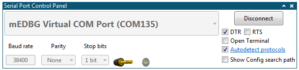
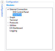
- Open the Serial Port Control panel found under External Connection in the Modules section of the Configuration tab in Data Visualizer
- Select the correct COM port corresponding to the connected kit
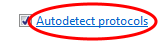
- Make sure Autodetect protocols option is checked and the Parity and Stop bits configurations are set according to the target application. The Baud rate will be detected automatically.
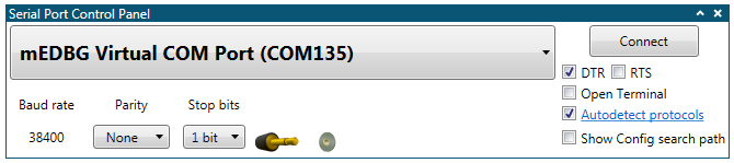
- Click Connect
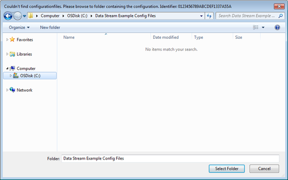
- If Data Visualizer cannot find the configuration files for the detected Auto-Configuration ID it will show a pop-up asking for the path to the configuration files. Browse to the folder where the configuration files reside and click OK
After connecting and detecting the Auto-Configuration ID the Data Visualizer should create a Data Stream Control Panel and a Dashboard I/O looking something like the image below.
The Graph element shows a running sawtooth signal which represents the counter continuously counting up until it wraps. The Signal element shows the state of the push button on the ATtiny104 Xplained Nano board. Pushing the button changes the color of the Signal element from red to green.
Expanding the Data Stream Control Panel by clicking the down arrow to the right in the panel shows the content of the automatically configured Data Stream.

The stream has two sources, one for the counter value and one for the button state.

Expanding the Serial Port Control Panel shows that Data Visualizer detected the baud rate to be 38400.